AI Infrustructure and compute optimization

Overview

The explosive growth of artificial intelligence, from large language models like GPT-4 to generative image systems like DALL-E, is often depicted as a triumph of algorithms and data. While these are crucial ingredients, the unsung hero of this revolution is the underlying AI infrastructure—the specialized hardware, software, and orchestration layers that transform mathematical models into functioning, scalable applications.

This piece explores the critical domain of AI Infrastructure and Compute Optimization. It moves beyond the model code to examine the foundational stack that makes modern AI possible. We define AI infrastructure as the integrated ecosystem of computational resources, data pipelines, networking, and software frameworks required to develop, train, deploy, and maintain AI systems at scale. Compute optimization is the discipline of maximizing the efficiency, speed, and cost-effectiveness of this infrastructure throughout the AI lifecycle.

The journey from a prototype to a production AI system is fraught with computational challenges:

The Training Bottleneck: Training state-of-the-art models can require thousands of specialized accelerators (GPUs, TPUs) running for weeks, consuming megawatts of power and millions of dollars.

The Deployment Dilemma: Serving these massive models to millions of users with low latency demands a completely different optimization profile than training.

The Resource Scarcity: With global demand for AI compute far outstripping supply, simply throwing more hardware at the problem is neither feasible nor economical.

Therefore, optimization is no longer a niche concern; it is a core business imperative. This involves a multi-layered approach:

(1). Hardware Efficiency: Leveraging specialized chips (GPUs, TPUs, NPUs) and understanding their memory hierarchies, interconnect technologies (NVLink, InfiniBand), and optimal configuration.

(2). Software Orchestration: Utilizing frameworks (PyTorch, TensorFlow), compilers (XLA, OpenAI Triton), and kernels to ensure hardware is fully saturated with minimal idle time.

(3). Systems Architecture: Designing scalable, fault-tolerant clusters for distributed training and inference, often across hybrid cloud environments.

(4). Algorithmic & Model-Level Optimization: Techniques like mixed-precision training, model pruning, quantization, and distillation that drastically reduce computational load without proportional losses in accuracy.

Intended Audience

This piece is designed for technical professionals, decision-makers, and enthusiasts who are involved in building, deploying, or managing AI systems and need to understand the infrastructure that powers them.

(1). ML Engineers & AI Researchers: Practitioners who write model code and face the direct challenges of long training times, out-of-memory errors, and slow iteration cycles. They will gain insights into how to structure their workloads and leverage tools to maximize the productivity of their compute resources, moving faster from research to production.

(2). Infrastructure & DevOps Engineers: Professionals responsible for provisioning, maintaining, and scaling the clusters and cloud environments where AI workloads run. This content will help them understand the unique demands of AI workloads (vs. traditional web services) and guide the design of robust, efficient, and cost-effective platforms for their data science teams.

(3). Technical Leaders & Architects: CTOs, VPs of Engineering, and Solutions Architects who make strategic decisions about technology investments, cloud strategy, and platform choices. This overview will equip them with the framework to evaluate infrastructure trade-offs, plan for scale, and align compute strategy with organizational AI goals.

(4). Cloud & Hardware Enthusiasts: Individuals keen on understanding the cutting-edge developments in accelerated computing, interconnect technology, and how cloud providers (AWS, Google Cloud, Azure) are structuring their AI/ML service offerings.

(5). Product Managers for AI-Powered Products: PMs who need to understand the infrastructural constraints and costs that influence model capabilities, deployment feasibility, latency, and ultimately, user experience and roadmap planning.

Prerequisite Knowledge: The article assumes a foundational understanding of what machine learning and deep learning are, and a high-level familiarity with concepts like neural network training and inference. It does not require expert-level hardware or systems knowledge, as it aims to build that bridge from first principles to current best practices.

1.1 Basics of Artificial Intelligence workload

AI Workloads: The Fundamental Dichotomy of Training vs. Inference

Understanding the distinction between training and inference is the essential first step in designing efficient AI infrastructure. These two phases represent fundamentally different computational challenges, each with unique performance characteristics, resource requirements, and optimization strategies.

The Two Pillars of the AI Lifecycle

(1). Training Training is the process of creating the AI model itself—teaching it patterns from data.

What happens

A model's architecture ( a neural network with millions or billions of parameters) is initialized, typically with random values.

The model is fed massive volumes of labeled data (like images with descriptions, text sequences, game states).

Through iterative optimization (primarily backpropagation), the model's internal parameters are adjusted to minimize a loss function—the difference between its predictions and the correct answers.

This process runs continuously for hours, days, or even weeks until the model achieves satisfactory accuracy.

*Key characteristics Compute-Intensive: Requires immense, sustained computational power, primarily floating-point matrix operations.

Batch-Oriented: Processes huge batches of data in parallel to compute stable gradient updates.

Stateful & Iterative: Maintains the evolving state of the model parameters across thousands or millions of iterations.

High-Precision: Typically uses 32-bit (FP32) or mixed 16/32-bit (FP16/BF16) precision to ensure stable convergence.

Cluster-Scale: Often distributed across hundreds or thousands of accelerators (GPUs/TPUs) working in concert.

(2). Inference Inference is the process of using a trained model to make predictions on new, unseen data.

What Happens:

A trained, fixed model (its parameters are now frozen) receives an input (e.g., a user's prompt, a new image, a sensor reading).

The model performs a forward pass through its network to produce an output (e.g., generated text, a classification, a forecast).

The result is returned to the user or application.

Key Characteristics:

Latency-Sensitive: Often needs to meet strict response-time Service Level Objectives (SLOs), especially for interactive applications (e.g., chatbots, real-time recommendations).

High-Throughput: May need to serve millions of requests per second globally (e.g., spam detection, photo tagging).

Stateless: The model parameters do not change; each request is independent.

Precision-Optimized: Often uses lower precision (INT8, FP16) to speed up computation and reduce memory usage without significant accuracy loss.

Cost-Efficient: Must run continuously 24/7; operational cost and energy efficiency become primary concerns.

Aspect	Training Workloads	Inference Workloads
Primary Goal	Accuracy / Convergence	Latency & Throughput
Compute Pattern	Long-running, batch-parallel, communication-heavy	Short-burst, request-parallel, communication-light
Hardware Focus	Peak FLOPs & High-Bandwidth Interconnects	Memory Bandwidth, Low-Latency I/O, & Energy Efficiency
Critical Metric	Time-to-Train (e.g., hours to train GPT-4)	P99 Latency & Queries Per Second (QPS) per Dollar
Precision	FP32, Mixed (FP16/BF16) for stability	INT8, FP16, sometimes FP32 for sensitive tasks
Scale	Large, expensive clusters used intermittently	Many smaller, distributed deployments, running constantly
Failure Tolerance	Checkpointing; can restart from last save	Must be highly available; failures directly impact users

Training is a scientific endeavor; inference is an engineering one. You build infrastructure once for a training run, but you build it for resilience and scale for inference.

This dichotomy informs every subsequent decision in AI infrastructure:

You cannot design a cost-effective inference system using the same principles as your training cluster.

Purchasing decisions, cloud vendor choices, and software frameworks must align with which phase you are optimizing for.

The emerging practice of MLOps is largely about managing the transition between these two worlds—taking a model from the experimental, training-focused environment to a stable, scalable, inference-serving production system.

Why is AI compute intensive?

Modern AI is computationally intensive due to its core nature and the pursuit of unprecedented capability. Fundamentally, deep learning performs trillions of matrix multiplications across neural networks with billions to trillions of parameters. This scale is driven by empirical Scaling Laws, which show that model performance directly correlates with model size, dataset size, and compute used for training, creating an inevitable race toward larger models.

The dominant transformer architecture compounds this with quadratic computational complexity for its attention mechanism, making longer context windows exponentially more expensive. Furthermore, the iterative process of training requires processing massive datasets multiple times, performing forward passes, backward propagation, and optimizer updates.

A critical bottleneck is the "memory wall." Moving model weights and data between GPU memory, system RAM, and storage is vastly slower than the computation itself, often leaving powerful processors idle while waiting for data.

Difference between traditional software workloads and AI workloads

Modern AI represents a paradigm shift in computing, demanding entirely new infrastructure approaches. At its core, AI splits into two distinct phases with divergent requirements: Training (the compute-intensive, stateful "learning" phase) and Inference (the latency-sensitive, stateless "application" phase). Training consumes weeks of specialized cluster time to iteratively adjust billions of parameters, while inference serves predictions at scale, where cost-per-query and response time are critical.

The astronomical compute demands stem from fundamental factors: AI executes massively parallel matrix operations across neural networks with billions of parameters, governed by empirical scaling laws that show capability grows predictably with compute investment. The transformer architecture's quadratic attention complexity and the relentless "memory wall"—where moving data between storage and compute cores becomes the primary bottleneck—compound this intensity. Unlike traditional software, AI workloads are statistical, hardware-specific, and computationally bound, requiring specialized accelerators (GPUs/TPUs) rather than general-purpose CPUs.

This creates a stark contrast with traditional enterprise workloads. Where conventional software is I/O-bound, predictable, and horizontally scalable, AI is compute-bound, probabilistic, and requires monolithic scaling for training. The infrastructure mindset must shift from maximizing general cluster utilization to maximizing accelerator saturation and minimizing data movement. Performance metrics evolve from request latency to time-to-train and tokens-per-second-per-dollar.

Optimization therefore operates on three fronts:

(a). Hardware: Matching specialized chips (H100s for training, Inferentia for inference) to their ideal workloads.

(b). Software: Using kernel fusion, mixed precision training, and model quantization to reduce computational and memory overhead.

(c). Systems: Designing distributed training strategies (data/model parallelism) and inference serving systems with dynamic batching.

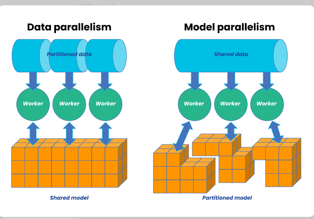
Data Parallel and Model Parallel computation

Aspect	Data-Parallel	Model-Parallel
What’s Split	Data (batches)	Model (layers / tensors)
What’s Copied	Full model on each device	Data batch to all devices
Communication	Gradient synchronization (All-Reduce)	Activation passing between devices
When Used	Model fits in single GPU memory	Model too large for single GPU
Scaling Limit	Batch size & gradient sync overhead	Pipeline “bubbles” & communication latency
Complexity	Lower – easier to implement	Higher – requires careful partitioning

How they work

Data parallel

[Batch of 64] → Split → [GPU1: 16 samples] → Compute Gradients [GPU2: 16 samples] → Compute Gradients
[GPU3: 16 samples] → Compute Gradients [GPU4: 16 samples] → Compute Gradients ↓ Average Gradients (All-Reduce) ↓ Update All Model Copies Together

Each GPU: Has complete model copy + different data slice

Sync point: Gradients averaged after each iteration

Best for: CNN, BERT-sized models (single GPU memory)

Model parallelism

Two Main Types:

1. Pipeline Parallel (Vertical Split): GPU1: Layers 1-4 → GPU2: Layers 5-8 → GPU3: Layers 9-12 [Batch 1] → → → Output [Batch 2] → [Bubble] → → Output ← Idle time! [Batch 3] → → [Bubble] → Output ← More idle time!

2. Tensor Parallel (Horizontal Split): GPU1: First half of layer computation GPU2: Second half of layer computation ↓ Sync activations after EACH layer operation

1.2 Fundamentals of computing infrastructure

What "compute" means in AI.

"Compute" in AI refers to the specialized hardware and mathematical capacity required to train and run neural networks—specifically the ability to perform massive parallel matrix operations efficiently. Unlike general computing, AI compute prioritizes throughput over latency and requires hardware fundamentally different from traditional CPUs.

Core hardware comparison

Hardware Type	Primary Strength	AI Role	Key Limitation	Best For
CPU	Complex logic, versatility	Controller, data prep	Poor parallelism	Light inference, orchestration
GPU	Massive parallelism	AI workhorse	Power consumption	Training & flexible inference
TPU	Matrix math efficiency	Google ecosystem	Software lock-in	TensorFlow workloads
AI ASICs	Specialized efficiency	Task-specific acceleration	Inflexibility	High-volume inference

The memory hierarchy- the true bottleneck AI compute isn't just about calculations—it's about moving data efficiently through a memory pyramid:

[Slowest/Largest] [Fastest/Smallest] ↓ ↓ Storage (PB) ↓ ↓ On-Chip Cache (MB) System RAM (TB) ↓ ↓ GPU Memory (GB) ← BOTTLENECK! PCIe Bus ↓ ↓ Compute Cores Data Movement > Computation

Memory Bandwidth Reality Check: CPU DDR5 RAM: ~100 GB/s

PCIe 5.0 (CPU↔GPU link): ~128 GB/s ← Choke point!

NVIDIA H100 HBM3: 3.35 TB/s (33× CPU speed)

Google TPU v4: 1.2 TB/s chip-to-chip

Why traditional CPUs fail at AI

CPUs are optimized for sequential, branch-heavy code—exactly what AI isn't:

CPU Design	AI Workload Reality	Mismatch Impact
Few cores (8-64)	Needs 1000s of parallel ops	< utilization
Complex control logic	Predictable data flow	Wasted silicon
Optimized for latency	Needs throughput	Poor efficiency
General-purpose	Highly specialized	Energy inefficient

A GPU's 10,000+ simple cores executing the same instruction on different data (SIMD) matches AI's mathematical regularity perfectly.

AI compute has evolved from "anything that runs code" to highly specialized hardware ecosystems optimized for matrix mathematics. Success requires matching:

Hardware architecture to workload characteristics

Memory hierarchy to model size

Software ecosystem to team expertise

Deployment model to economic constraints

The future belongs not to the fastest individual chip, but to the most cohesive hardware-software stack that minimizes data movement, maximizes utilization, and provides predictable scaling from prototype to planetary deployment.

Memory hierarchy:AI data pathway

The memory hierarchy is a tiered system that balances speed, capacity, and cost. For AI, managing this hierarchy is the primary performance challenge.

Fastest/Smallest/Expensive → Slowest/Largest/Cheapest

Registers (KB): Inside the processor. 1 cycle access. Holds data being computed right now.

Cache (MB): On-chip SRAM. L1/L2/L3, ~10-100 cycles. Holds recent/frequent data (model weights, activations).

RAM/VRAM (GB/TB): System/GPU memory. ~100-500 cycles. Holds the working set: full model, batches, gradients. Bottleneck for AI—must feed the compute cores fast enough.

Storage (TB/PB): SSD/HDD/NAS. ~10,000+ cycles. Holds datasets, checkpoints, model archives.

The Core Problem in AI: The Memory Wall Compute cores are thousands of times faster than fetching data from RAM. A GPU tensor core can perform an operation in nanoseconds but may wait microseconds for weights to arrive.

AI-Specific Challenge:

Training: Must fit model + optimizer states + activations in fast memory (GPU VRAM) or performance crashes.

Inference: Latency dominated by loading weights from VRAM to registers. Larger models that don't fit in VRAM must swap from slower RAM (via PCIe), killing speed.

Solution Focus: Minimize movement up the hierarchy. AI chip design focuses on massive bandwidth (HBM).

Storage Types for AI

Storage is the slowest tier in the memory hierarchy but holds the massive datasets and model checkpoints for AI. Choosing the right type directly impacts training throughput and cost.

Type	Speed	Best for AI	Key Limitation
HDD (Hard Disk Drive)	Slow (100–200 MB/s)	Cold storage for archived datasets and logs	High latency, poor random access
SSD SATA (Solid State Drive)	Moderate (500–600 MB/s)	Active datasets and frequent checkpoints	SATA bus bottleneck
NVMe SSD (Non-Volatile Memory Express)	Fast (3–7 GB/s)	High-performance training pipelines	Higher cost per TB
NVMe over Fabrics (NVMe-oF)	Extreme (network-speed)	Multi-node training with shared storage	Complex setup, expensive

For AI Workloads:

Training: Use NVMe SSDs for your active dataset drive. Sequential reads of training files benefit massively from NVMe speed.

Checkpointing: NVMe or fast SATA SSD to minimize the time GPUs sit idle while saving model state.

Archival: HDD arrays for cost-effective petabyte-scale storage of raw data and old model versions.

Evaluating AI compute requires metrics beyond traditional computing benchmarks. Here are the critical measures that determine real-world performance and efficiency.

3 Computer architecture for AI

This section examines the specialized hardware that powers modern AI workloads. Today, the landscape emphasizes massive parallelism, ultra-high-bandwidth memory (HBM), low-precision compute for efficiency, and tight interconnects to overcome the memory wall and enable exascale-scale training and low-latency inference.

2.1 CPU Architecture

Role of CPUs in AI systems

CPUs serve as orchestrators rather than primary compute engines. They handle data preprocessing, I/O coordination, control flow, scheduling, and lightweight inference tasks. In AI clusters, CPUs manage OS-level operations, network communication, and coordination between accelerators.

SIMD, multithreading, and vectorization

Modern CPUs leverage SIMD (Single Instruction, Multiple Data) via AVX-512 or AMX instructions, enabling vectorized operations on small batches or non-matrix workloads. Multithreading (via many cores and hyper-threading) supports concurrent data loading and preprocessing. Vectorization accelerates element-wise operations, but limited core counts and lower parallelism restrict CPUs to auxiliary roles.

CPU bottlenecks in AI workloads

CPUs suffer from few cores (typically 64–128), complex branch-heavy logic, and lower memory bandwidth (~100–200 GB/s DDR5). They deliver poor utilization on matrix-heavy AI tasks, leading to energy inefficiency and idle time. The mismatch with AI's predictable, throughput-oriented nature makes general-purpose CPUs unsuitable as primary accelerators.

2.2 GPU Architecture

Why GPUs dominate AI

GPUs excel due to thousands of simple cores executing SIMD instructions in lockstep, perfectly matching AI's regular matrix multiplications and massive parallelism. They provide high throughput for training and flexible inference, with mature ecosystems (CUDA, ROCm).

CUDA cores, tensor cores

CUDA cores handle general-purpose parallel compute (FP32/FP64). Tensor Cores are specialized matrix units for accelerated deep learning. In NVIDIA's Blackwell architecture (dominant in 2026), fifth-generation Tensor Cores support FP4, FP6, FP8, and NVFP4 formats, delivering massive gains: e.g., B200 offers ~9–18 PFLOPS FP4 (dense/sparse), with 2× attention acceleration and micro-tensor scaling via the second-generation Transformer Engine.

GPU memory (HBM, VRAM)

High-Bandwidth Memory (HBM3e) is critical. Blackwell GPUs feature 192 GB HBM3e per B200 (up to 8 TB/s bandwidth), far surpassing Hopper's H100/H200 (~3.35–4.8 TB/s). This addresses the memory wall by feeding tensor cores rapidly, enabling larger models/batches without excessive swapping.

GPU scheduling and parallelism GPUs use massive thread-level parallelism (warps of 32 threads) and streaming multiprocessors (SMs) for concurrent execution. Features like cooperative groups, warp-level primitives, and MIG (Multi-Instance GPU) enable efficient partitioning. NVLink 5 and NVSwitch provide ultra-high interconnect bandwidth (e.g., 130 TB/s domains in NVL72 racks), minimizing communication overhead in multi-GPU setups.

2.3 AI Accelerators TPUs and NPUs

TPUs : Systolic arrays optimized for matrix multiply. TPU v5p delivers ~459 TFLOPS BF16 per chip (95 GB HBM2e, 2.765 TB/s). Newer generations like TPU v7 (Ironwood) reach ~4,614 TFLOPS BF16/FP8, 192 GB memory, and ~7.37 TB/s bandwidth, excelling in Google's ecosystem for training and inference.

*NPUs (Neural Processing Units): Integrated in client/edge devices (e.g., Intel Core Ultra, AMD Ryzen AI, Qualcomm) for efficient on-device inference. They focus on low-power, quantized workloads (INT8/FP16).

ASICs for AI

Application-Specific Integrated Circuits deliver peak efficiency for fixed workloads. Examples:

Groq LPUs for ultra-low-latency inference (~185 tok/s, sub-ms TTFB). Cerebras WSE-3 (wafer-scale) for massive on-chip memory and fast trillion-parameter training. AWS Trainium/Inferentia, Tenstorrent, SambaNova RDUs, and Etched transformers target specific domains (e.g., inference efficiency, reconfigurable dataflow). ASICs trade flexibility for 5–30× better perf/W or latency vs. GPUs in targeted scenarios.

FPGA-based acceleration

FPGAs offer reprogrammability for custom datapaths (e.g., low-precision inference, sparse tensors). AMD (Xilinx) Versal and Intel Agilex/Stratix families integrate AI engines for adaptive acceleration in data centers, edge, and automotive. They suit dynamic workloads or when full ASIC redesign is impractical, though they lag GPUs/ASICs in raw throughput for standard transformers.

2.4 Memory Architecture Memory architecture is the dominant factor in AI performance as of February 2026. The "memory wall" persists: compute capabilities (FLOPS) have scaled dramatically, but memory bandwidth and capacity improvements lag, leaving accelerators memory-bound for most deep learning workloads—especially inference and large-model training. The roofline model illustrates this: performance is capped by the minimum of peak compute and (bandwidth × arithmetic intensity). Low arithmetic intensity (operations per byte moved) pushes workloads into the memory-bound region, where extra FLOPS yield no gains.

Cache coherence

Cache coherence ensures consistent views of shared data across caches in multi-processor systems. In single-GPU setups, intra-GPU coherence (L1/L2 caches) is hardware-managed. In multi-GPU clusters:

NVIDIA NVLink (Gen 5/6 in Blackwell/Rubin) and NVLink-C2C provide hardware cache coherence for GPU-GPU and CPU-GPU sharing. This enables coherent unified address spaces (e.g., Grace-Blackwell Superchip treats LPDDR and HBM as one coherent pool). Benefits include direct load/store across devices, reduced explicit transfers, and atomic operations without software overhead. Trade-off: coherence traffic consumes interconnect bandwidth; protocols optimize via directories and snoop filters.

Unified memory

Unified memory (CUDA-managed) creates a single virtual address space accessible from CPU and GPU, with runtime handling page migrations via faults.

Emerging: Extended GPU memory pools (e.g., via NVLink fabrics) allow addressing terabytes coherently.

Memory bottlenecks in deep learning

The memory wall dominates:

Training: Model parameters, activations, gradients, and optimizer states exceed fast memory (HBM), forcing spills to slower system RAM/PCIe/storage → idle compute cores. Inference (decode phase): Low arithmetic intensity (~1–10 FLOPs/byte for autoregressive generation); KV cache and weights dominate bandwidth demand. Per-token latency is often HBM-bound, not compute-bound. Current accelerators: NVIDIA Blackwell B200/B300 (192–288 GB HBM3e, ~8 TB/s bandwidth), Google TPU v7/Ironwood (~192 GB, ~7.37 TB/s), but even these saturate on frontier models (trillions of parameters, long contexts). HBM supply/packaging remains a systemic constraint.

Compute-to-memory ratio

Also called arithmetic intensity or operational intensity (FLOPs/byte moved from memory).

High ratio → compute-bound (ideal for peak FLOPS utilization). Low ratio → memory-bound (roofline knee shifts right as compute grows faster than bandwidth). In transformers: GEMM operations achieve high intensity; attention and decode phases drop low (quadratic attention but linear KV cache access). 2026 reality: Many AI workloads fall below 100–500 FLOPs/byte thresholds needed to saturate modern HBM → emphasis shifts to bandwidth, larger on-chip caches (e.g., Blackwell's expanded L2), kernel fusion, and prefetching over raw FLOPS. Mitigation: Quantization (FP4/FP8/NVFP4), sparsity, larger HBM stacks, and coherent multi-chip fabrics to boost effective intensity.

3 Operating System and system: The foundation of AI compute optimization

operating systems and systems software form the critical foundation where compute optimization truly begins. This layer transforms raw hardware into a predictable, efficient platform for AI workloads, managing the complex interplay between parallel computations, memory hierarchies, and I/O patterns that define modern machine learning.

The Multifaceted Role of the Operating System in AI

Thread Management: The OS must efficiently manage hundreds of framework threads, using CPU pinning to bind critical threads to dedicated cores. This prevents oversubscription and cache thrashing for key operations like gradient synchronization.

Memory Management: The OS must minimize swapping and fragmentation for massive model weights and datasets. Using huge pages (2MB/1GB) instead of 4KB pages drastically reduces TLB misses. This requires coordination with GPU memory allocators to prevent fragmentation.

I/O Handling: AI training has unique I/O patterns: sequential reads of datasets and burst writes of large checkpoints. The OS scheduler must optimize read-ahead caching for data and prioritize low-latency writes. The page cache must be carefully sized to balance data loading and memory for model weights.

Linux

Why Linux Dominates AI Infrastructure

Linux’s near-total dominance in AI data centers comes down to control, performance, and scalability at the systems level.

1. Kernel-Level Control

Linux allows deep customization that proprietary OSes don’t:

Kernel tuning for AI workloads (scheduler behavior, I/O paths)

Zero-copy data movement (mmap, direct I/O) to remove data-loading bottlenecks

Fine-grained scheduling control for latency-sensitive training and communication tasks

2. NUMA and Hardware Topology Awareness

Modern AI servers are NUMA systems:

Linux provides explicit NUMA control (numactl, NUMA-aware allocators)

Memory and CPU affinity reduce cross-node latency (often 2–3× slower otherwise)

Critical for GPU workloads: bind CPUs, memory, and GPUs based on PCIe/NVLink topology

3. GPU-Optimized Kernels and I/O

Production AI systems rely on Linux variants with:

High-performance async I/O (io_uring)

GPU-aware scheduling and memory management

Stable handling of GPU memory pressure and oversubscription

4. Containers and Resource Isolation

Linux primitives power all AI container platforms:

cgroups and namespaces enable isolation of CPU, memory, and I/O

Essential for multi-tenant training clusters

High-performance setups minimize virtualization overhead (bare-metal containers, lightweight runtimes)

The Final 10–20%: Precision Resource Management

This is where good systems become great.

CPU Isolation and Pinning

Dedicated cores for training, data loading, and communication threads

isolcpus, cpuset, taskset eliminate scheduler jitter

Enables predictable, low-latency synchronization

GPU-Aware Scheduling

Allocation based on NVLink and PCIe topology

Fractional GPU sharing where appropriate (MIG, vGPU)

Automated discovery and scheduling in production clusters

Intelligent Memory Management

Avoid naive memory caps that trigger OOM kills

Separate working memory from transient buffers (e.g., checkpoints)

Spill to fast storage instead of crashing under pressure

Power and Thermal Control

Dynamic frequency scaling aligned with workload phases

Proactive thermal management avoids throttling

Small per-node gains compound massively at scale

AI performance isn’t decided by models or hardware alone. The OS is a performance multiplier.

Linux enables:

Higher utilization

Predictable latency

Lower operational cost at scale

At cluster sizes where GPUs cost millions, even single-digit efficiency gains matter. That’s why elite AI teams treat systems software as a first-class discipline, not an afterthought.

4. AI Frameworks & Runtime Systems

This section bridges software abstractions to hardware acceleration. Modern deep learning frameworks define models and control execution, while runtime systems and compilers optimize the compute graph for efficient mapping to GPUs, TPUs, and other accelerators—critical for saturating hardware and minimizing idle time.

4.1 Deep Learning Frameworks

TensorFlow architecture

TensorFlow uses a dataflow graph model where computations are nodes (operations) and edges are tensors. It supports both eager execution (default since TF 2.x for intuitive debugging) and graph mode (via tf.function or tf.Graph for optimization). Keras provides a high-level API for rapid model building. The runtime compiles graphs for distributed execution across CPUs, GPUs, and TPUs, with strong production focus on scalability and deployment.

PyTorch execution model

PyTorch defaults to eager execution: operations execute immediately as Python code runs, building the computation graph dynamically ("define-by-run"). This enables natural debugging, dynamic control flow, and rapid prototyping. For production, torch.compile or TorchScript converts code to an optimized graph, enabling fusions and kernel specialization.

Static vs Dynamic Computation Graphs

Aspect	Static Graphs (e.g., TensorFlow graph mode, TorchScript)	Dynamic Graphs (e.g., PyTorch eager, TF 2.x eager)
Definition	Define-then-run: Graph built upfront, then executed	Define-by-run: Graph built on-the-fly during execution
Flexibility	Lower; fixed structure, harder for variable inputs/control flow	Higher; supports dynamic shapes, loops, conditionals natively
Debugging	More complex (requires tracing compiled graph)	Easier (standard Python debugging tools)
Optimization Potential	Higher: Full-graph view enables aggressive fusions, constant folding	Good with compilation (e.g., torch.compile); runtime overhead otherwise
Performance	Typically faster in production after compilation	Competitive with modern compilers; eager can be slower without optimization
Use Case	Deployment, large-scale training/inference	Research, prototyping, dynamic models

4.2 Compute Graph Optimization

These techniques reduce kernel launches, memory traffic, and redundant computation by transforming the graph before hardware execution.

Operator fusion — Combines sequential ops (e.g., Conv + BatchNorm + ReLU) into a single kernel, eliminating intermediate tensor materialization and reducing memory bandwidth pressure.

Kernel optimization — Custom or auto-tuned kernels (via Triton, CUTLASS) maximize hardware utilization; includes tiling, vectorization, and precision-specific implementations.

Graph pruning — Removes redundant nodes, constant folding, dead-code elimination, and shape inference to simplify the graph.

Lazy vs eager execution — Eager: immediate op dispatch (flexible but higher overhead). Lazy: defers execution to build full graph for holistic optimization (e.g., via torch.compile or XLA), enabling fusions and better scheduling.

4.3 Runtime Systems

CUDA runtime

NVIDIA's low-level API for GPU programming. Manages memory allocation, kernel launches, streams, and events. Frameworks like PyTorch and TensorFlow use it under the hood for direct GPU control; torch.cuda or tf.device provide abstractions.

XLA (Accelerated Linear Algebra)

Google's open-source domain-specific compiler (part of OpenXLA) that takes graphs from TensorFlow, JAX, or PyTorch (via torch_xla) and generates optimized kernels for CPUs, GPUs, and TPUs. It performs aggressive fusions, layout optimizations, and hardware-specific codegen, often yielding 20–50% speedups on matrix-heavy workloads.

ONNX Runtime

Cross-framework inference engine for ONNX models (exported from PyTorch, TensorFlow, etc.). Applies graph optimizations (fusion, constant folding), quantization, and execution providers (EPs) for hardware acceleration (CUDA, TensorRT, DirectML, etc.). Supports training acceleration and model compression for efficient deployment.

TensorRT

NVIDIA's high-performance inference SDK. Converts models (via ONNX or direct import) into optimized engines with layer fusion, precision calibration (FP16/INT8/FP8), dynamic shapes, and KV-cache optimizations for transformers. Excels in low-latency, high-throughput serving on GPUs, especially for LLMs.

5. Data Pipelines & Input Optimization

Many large-scale AI training jobs are bottlenecked by data input rather than GPU compute. Underutilized GPUs (often less than 30% utilization) signal that the system is starved for data, not compute-limited. Optimizing the data pipeline is usually the highest-leverage fix.

5.1 Data Loading Bottlenecks

I/O vs compute imbalance

Modern GPUs process batches in milliseconds, but loading and preprocessing a batch from storage can take seconds. This creates a pipeline where compute is idle waiting for I/O. The classic symptom is GPU utilization dropping sharply during training epochs while CPU and disk/network activity spike. The effective throughput is limited by the slowest stage.

Disk vs network bottlenecks

Local NVMe SSDs deliver 3–7 GB/s sequential reads, but many training jobs use network-attached storage.

Local disk: Fast (low latency, high bandwidth), but capacity is limited and scaling across nodes is hard.

Network storage: Object stores (S3) or distributed file systems introduce 10–100× higher latency and 5–50× lower bandwidth per client. Even with 100 Gbps links, effective throughput per node often falls to 100–500 MB/s due to protocol overhead, contention, and small-object reads.

5.2 Data Pipeline Optimization

Prefetching

Overlap data loading with model computation. Frameworks like PyTorch DataLoader (num_workers > 0, prefetch_factor > 1) and TensorFlow tf.data (prefetch) automatically load the next batch while the current batch is being processed. Effective prefetch depth is usually 2–4 batches.

Caching

Keep hot datasets in memory or fast local storage.

In-memory caching (RAM): Ideal for small-to-medium datasets (< GPU memory × nodes). Local SSD caching: Use tools like Alluxio, JuiceFS, or PyTorch torch.utils.data.dataset.Dataset with custom caching. Persistent caching layers (e.g., Redis, Memcached) for shared datasets across jobs.

Parallel data loaders

Use multiple worker processes/threads to saturate I/O bandwidth.

PyTorch: num_workers=8–32 (rule of thumb: 4–8 per GPU). TensorFlow: tf.data with num_parallel_calls=AUTOTUNE and interleave. Watch for memory thrashing and CPU contention—profile with nvidia-smi, htop, and iotop.

Compression strategies

Reduce I/O volume at the cost of CPU cycles for decompression.

On-disk: Zstandard (zstd), Blosc, or LZ4—fast decompression, good ratios (2–4×). In-flight: Use compressed formats (WebDataset shards with tar + zstd, TFRecord with gzip). Trade-off: Compression ratio vs decompression throughput. Zstd level 3–5 is often optimal for training.

5.3 Storage Systems for AI

Object storage

S3-compatible (AWS S3, GCS, MinIO, Ceph). Pros: Virtually unlimited scale, durability, pay-for-use. Cons: High first-byte latency (10–100 ms), lower throughput per connection, small-object penalty. Best for: Cold/archival data, multi-region access, or when using sharded formats (WebDataset, TFRecord) with prefetching.

Distributed file systems

Lustre, BeeGFS, WEKA, VAST, HDFS, or GPFS. Pros: High aggregate bandwidth (10–100 GB/s per node), POSIX compatibility, low latency for small reads. Cons: Expensive hardware, complex management, single-cluster scale limits. Best for: High-performance training clusters where local-like performance is needed at scale.

Local vs remote storage trade-offs

Local NVMe: Lowest latency, highest bandwidth, simplest. Use when dataset fits on-node or can be replicated. Remote: Enables massive scale and elasticity, but requires aggressive prefetching, caching, sharding, and sometimes dedicated data-loading nodes. Rule of thumb: If data-loading time > 20–30% of epoch time, move toward local caching or high-performance distributed storage.

6. Distributed Computing for AI

Scaling AI training beyond a single GPU requires efficient distributed strategies. For trillion-parameter models, parallelism and low-overhead communication are essential to achieve high MFU (Model FLOPs Utilization).

6.1 Parallelism Strategies

Data parallelism (DP)

Replicates the full model on each device/GPU; splits the batch across workers. Each computes forward/backward on its mini-batch slice, then synchronizes gradients (typically via All-Reduce). Simple, scales well to hundreds of GPUs when model fits in memory. Bottleneck: gradient sync overhead grows with scale.

Model parallelism (MP) / Tensor parallelism (TP)

Splits model layers or tensors (e.g., weights in a linear layer) across devices. Devices compute parts of the same batch in parallel, communicating activations/gradients. Essential for models larger than single-GPU memory. Higher communication volume (activations vs gradients).

Pipeline parallelism (PP)

Splits model into sequential stages (e.g., groups of layers) across devices. Micro-batching overlaps computation to hide bubbles. Reduces memory per device but introduces pipeline bubbles and activation recomputation needs.

Hybrid parallelism

Combines DP + TP + PP (often called 3D parallelism). Data split across replicas, tensors across intra-node GPUs, pipeline across nodes. Enables scaling to thousands of GPUs (e.g., in DeepSpeed, Megatron-LM, FSDP). Optimal for frontier models.

6.2 Distributed Training

Parameter servers

Centralized (or sharded) servers hold model parameters. Workers push gradients and pull updates. Supports asynchronous training, fault-tolerant, but suffers from single-point bottleneck and higher latency for large models.

All-reduce algorithms

Decentralized: each worker computes local gradients, then collectives (e.g., ring All-Reduce, tree All-Reduce) aggregate them. Ring All-Reduce is bandwidth-optimal (constant time for large gradients). Dominant in modern synchronous training (e.g., NCCL, Horovod).

Communication overhead

Dominates at scale: gradients (~model size) must sync every step. All-Reduce bandwidth scales with N workers; latency-sensitive ops (small messages) hurt. Mitigations: gradient compression, overlapping comm/compute, sharded optimizers (ZeRO).

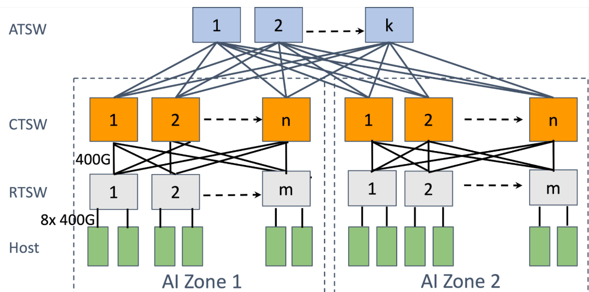
6.3 Networking for AI Compute

High-bandwidth interconnects

AI clusters use 200–800 Gbps per link (e.g., NVIDIA NDR InfiniBand, Ethernet with RoCEv2). Aggregate bandwidth per node: 8–16 links for 1.6–6.4 Tbps.

Latency vs throughput trade-offs

Throughput critical for large All-Reduce (gradients). Latency matters for small ops (activations in TP/PP). InfiniBand offers ~1 μs tail latency; well-tuned RoCE approaches it but can suffer congestion without PFC/ECN tuning.

RDMA

Remote Direct Memory Access bypasses CPU/kernel for zero-copy transfers. Enables low-latency, high-throughput collectives. Both InfiniBand and RoCE support RDMA; RoCE uses Ethernet hardware, cheaper but requires lossless fabric.

Network topology effects

Fat-tree or Clos for non-blocking bisection bandwidth. Poor topology (e.g., oversubscription) causes incast/congestion during collectives. Modern AI fabrics use rail-optimized designs (multiple NICs per host) for path diversity and fault tolerance.

7 Cloud AI Infrastructure

Cloud platforms dominate AI workloads due to elastic scaling, managed services, and access to the latest GPUs without CapEx. Key decisions revolve around control vs convenience and cost vs reliability.

7.1 Cloud Compute Basics

Virtual machines vs bare metal

VMs: Flexible, quick provisioning, multi-tenant isolation, oversubscription possible. Dominant for most training/inference (e.g., AWS p5/g6, GCP A3, Azure NDv5).

Bare metal: Direct hardware access, no hypervisor overhead, predictable performance, better for latency-sensitive or max-utilization jobs. Offered by AWS (rare), GCP Bare Metal, Azure (limited), or specialized providers (CoreWeave, Lambda Labs). Use when VM noise or hypervisor tax >5–10%.

Containers and virtualization

Containers (Docker) + orchestration (Kubernetes via EKS/GKE/AKS) enable portability and multi-tenancy. GPU support via device plugins (NVIDIA GPU Operator). Virtualization adds ~1–3% overhead but simplifies management. For AI: use containerized frameworks (PyTorch, TensorFlow) on managed K8s for reproducibility and autoscaling.

GPU instances

Major providers offer H100/A100/L40S/B200 equivalents:

AWS: p5 (H100), g6 (L4), p4d (A100) GCP: A3 (H100), A2 (A100), G2 (L4) Azure: ND H100 v5, NC A100 v4 Multi-GPU nodes (8×) common; interconnect via NVLink or InfiniBand. Spot/preemptible pricing critical for cost.

7.2 Cloud AI Services

Managed training platforms

Handle cluster provisioning, data loading, distributed training, checkpointing:

AWS SageMaker (Pipelines, Training Jobs, HyperPod for large clusters) Google Vertex AI (custom training, distributed jobs, TPUs) Azure ML (compute clusters, pipelines) Pros: built-in fault tolerance, experiment tracking, auto-scaling. Cons: vendor lock-in, sometimes higher cost than raw instances.

Managed inference services

Serverless or managed endpoints for production:

AWS Bedrock / SageMaker Endpoints Google Vertex AI Prediction Azure OpenAI / ML inference Support auto-scaling, A/B testing, monitoring. Ideal for variable traffic; pay-per-token or per-request.

Serverless AI

Functions + models (e.g., AWS Lambda + Bedrock, GCP Cloud Run, Azure Functions). Zero infrastructure for low-to-medium throughput inference. Cold starts and limits (memory/time) restrict large models.

7.3 Cost vs Performance Optimization

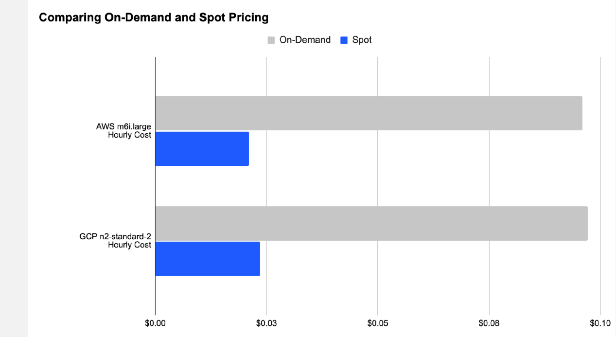
Spot instances

Preemptible capacity at 50–90% discount. AWS Spot, GCP Preemptible/Spot VMs, Azure Spot.

Savings: often 70–80% on GPUs Risk: 2-min warning (AWS), 30-sec (Azure/GCP); use checkpointing + fault-tolerant frameworks (DeepSpeed, FSDP). Best for: non-time-critical training, hyperparameter sweeps.

Autoscaling

Dynamic node count based on queue depth or GPU utilization (SageMaker, Vertex AI, Karpenter on EKS). Reduces idle costs; combine with spot for aggressive savings.

Right-sizing workloads

Match instance type to workload: memory-bound → high-memory GPUs; compute-bound → high-TFLOPS. Profile with nvidia-smi, nsight. Avoid over-provisioning (e.g., 8×H100 for batch size that fits on 4).

Cost-aware scheduling

Tools like AWS Instance Scheduler, Kubecost, or custom bin-packing place jobs on cheapest/available capacity. Reserve instances/Savings Plans for predictable baseline; fill with spot. Monitor with CloudWatch/Billing alerts.

9. Compute Optimization Techniques

Maximizing throughput, reducing memory footprint, and minimizing latency are critical for both training and inference at scale. These techniques often yield 2–10× gains when combined.

9.1 Model Optimization

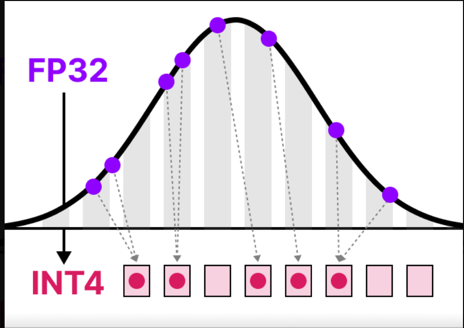
Quantization

Reduce precision of weights/activations (FP32 → FP16/INT8/INT4/FP8).

Post-training: Simple, ~4× memory reduction, 2–4× speedup on supported hardware. Quantization-aware training (QAT): Retrain with fake quant ops → minimal accuracy drop. Modern formats (AWQ, GPTQ, SmoothQuant) preserve quality at 4-bit for LLMs.

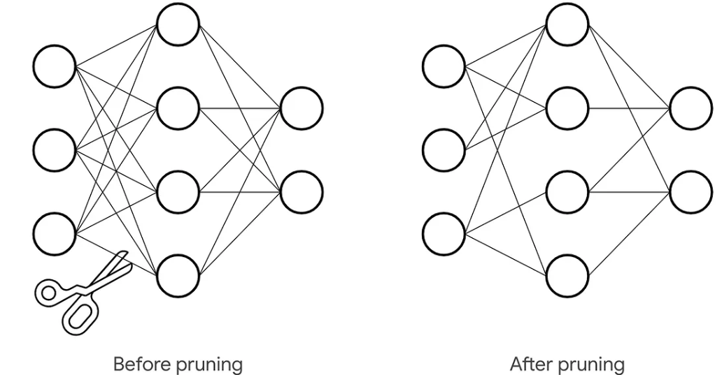
Pruning

Model Pruning is a compression technique where less important parameters (weights) or entire structural units (neurons, channels, layers) are removed from a neural network to reduce its size and computational cost.

The process relies on defining an importance criterion to select what to remove. Common criteria include:

Magnitude-based: Removing the smallest absolute weights, under the assumption they contribute least.

Gradient-based: Using gradient information from training to identify low-saliency parameters.

Pruning can be unstructured or structured:

Unstructured Pruning removes individual weights anywhere in the model, creating an irregular, sparse pattern. While it can achieve high compression rates, it often requires specialized software libraries and hardware to realize speedups, as standard GPUs are optimized for dense computations.

Structured Pruning removes larger structural components (e.g., entire neurons, filters, or attention heads). This results in a smaller, denser model that can achieve acceleration on standard hardware (like CPU/GPU) and is easier to deploy, though it may be less fine-grained than unstructured pruning.

Pruning is almost always performed as an iterative, gradual process, not a single drastic cut:

(1). Prune a small percentage of the model based on the chosen criterion.

(2). Fine-tune the remaining network to recover the accuracy lost from pruning.

(3). Repeat this cycle over several iterations until the target model size or sparsity is reached. This allows the network to adapt gradually, preserving more performance than one-shot pruning.

A well-pruned model can typically achieve 50–90% sparsity (i.e., 50–90% of its weights are zero) with a final accuracy loss of less than 1–2% compared to the original dense model, provided adequate fine-tuning or recovery training is performed. The final step often involves a final, longer fine-tuning phase on the full training dataset to maximize recovered performance.

9.2 Hardware-Aware Optimization

Mixed precision training

Use FP16/BF16 for most ops, FP32 for master weights/gradients/optimizer states.

Tensor Cores on Ampere+ deliver 2–8× speedup. Automatic via torch.amp / tf.keras.mixed_precision. Loss scaling prevents underflow.

Tensor cores utilization

Target matrix multiply ops (GEMM) that map to tensor cores.

Use shapes divisible by 8/16 (e.g., hidden size multiples). Frameworks auto-optimize; manual: fused kernels, avoid small reductions. BF16 preferred over FP16 for stability on Hopper+.

Memory-efficient models

Gradient checkpointing: Trade compute for memory (recompute activations). Activation recomputation, ZeRO-Offload, FlashAttention. Enable fitting 70B+ models on 8×80GB GPUs.

9.3 Inference Optimization

Batch sizing

Balance throughput vs latency.

Larger batches → higher throughput (better GPU utilization). Smaller batches → lower latency (critical for interactive use). Knee point often 8–32 for LLMs.

Model compilation

Torch.compile / torch dynamo → graph fusion, kernel selection. TensorRT / TVM / ONNX Runtime → optimized kernels, layer fusion, precision tuning. 1.5–3× speedup + lower memory.

Edge vs cloud inference

Cloud: High throughput, elastic scaling, latest GPUs (H100/B200). Use for heavy loads. Edge: Low latency, privacy, offline (mobile/embedded). Use quantized models (INT4/INT8), pruned/sparse, tiny models (MobileNet, NanoLLM). Trade-off: Edge → power/latency win; cloud → accuracy/scale win.

10. Energy Efficiency & Sustainability

Training large models requires enormous compute: weeks/months on thousands of GPUs, each performing trillions of operations per second.

10.1 Power Consumption in AI

Why AI consumes massive energy

Training large models requires enormous compute: weeks/months on thousands of GPUs, each performing trillions of operations per second.

NVIDIA H100: TDP 700W per GPU; full AI training nodes (8×H100) draw ~8–10 kW (actual measured often 18% below rated TDP). Frontier training runs: 10–50+ GWh per model (e.g., equivalents to powering thousands of homes for months). Inference: lower per query (~0.3 Wh for ChatGPT-like), but scales with billions of daily queries → MW-scale continuous draw. Key drivers: parameter count, dataset size, low utilization during I/O waits, cooling overhead (~30–50% of total power).

Data center power usage

Global data centers: ~415–460 TWh in recent years (~1.5% of electricity).

AI-accelerated servers drive fastest growth; projected 945–1,050 TWh by 2026–2030 (~3% global). US: data centers ~4–6% of electricity (2023–2025), potentially 8–12% by 2030. AI contribution: 10–50% of data center power by late 2020s; hyperscale campuses target 1–5 GW sites.

10.2 Green AI

Energy-efficient models

"Green-in-AI": design for efficiency from the start.

Quantization (INT4/FP8), pruning (50–90% sparsity), distillation (e.g., DistilBERT: 40% size, 97% performance). Efficient architectures (MobileNet-style depthwise convs, sparse models). Mixed precision + FlashAttention → 2–4× lower energy for same accuracy. Goal: shift from accuracy-only to accuracy-per-joule metric.

Carbon-aware scheduling

Shift non-urgent workloads (training, batch inference) to times/regions with low-carbon intensity (high renewables).

Tools: dynamic scaling on spot instances during solar/wind peaks. Reduces emissions 20–50% with no model changes. Frameworks: integrate grid carbon APIs (e.g., ElectricityMap) into schedulers (Kubernetes, Slurm).

Sustainable AI infrastructure

Hardware: higher perf/Watt chips (H100 → Blackwell/GB200: better ops per joule despite higher TDP). Data centers: liquid cooling (30–40% less energy), PUE less than 1.1, renewable PPAs (Google/Microsoft aim carbon-free 24/7). Edge inference: quantized models on low-power devices reduce cloud reliance. Circular: reuse hardware, embodied carbon tracking.

11. Security & Reliability in AI Infrastructure

Often ignored until a breach or outage costs millions. Frontier-scale AI systems demand zero-trust principles, robust isolation, and aggressive fault tolerance to maintain uptime and confidentiality.

11.1 Infrastructure Security

Secure model deployment

Use containerized inference (Docker + Kubernetes) with least-privilege RBAC, network policies, and API gateways (e.g., Kong, Istio) to enforce input/output filtering. Apply guardrails: prompt sanitization, output content filters, rate limiting to block prompt injection, jailbreaks, and data exfiltration (OWASP LLM Top 10). Zero-trust access: ephemeral credentials, just-in-time approval for model loading, no static API keys. Encrypt models at rest/transit; use secure enclaves (e.g., NVIDIA Confidential Computing) for sensitive workloads. Red team regularly; monitor for anomalous prompts/responses.

Data protection

Classify and encrypt training/inference data (AES-256 at rest, TLS 1.3 in transit).

Track provenance; verify integrity with hashing/signing to prevent poisoning or drift.

Privacy techniques: differential privacy, federated learning, data depersonalization for compliance (GDPR, EU AI Act).

Avoid sensitive data in prompts; use RAG with authorization checks.

11.2 Reliability & Fault Tolerance Checkpointing

Save model state (weights, optimizer, RNG) periodically to resilient storage (e.g., distributed FS like WEKA, object store with versioning).

Use sharded/distributed checkpointing (PyTorch Distributed, DeepSpeed, FSDP) for fast save/restore on 1000+ GPUs.

Balance frequency: too often → I/O bottleneck; too rare → high progress loss. Adaptive strategies (e.g., topology-aware, closed-loop) minimize overhead.

Enable non-blocking saves to avoid stalling training.

Failure recovery

Synchronous training stalls on single-node failure → resume from last checkpoint automatically (Slurm, Kubernetes job controllers, custom watchers).

Frameworks: DeepSpeed ZeRO + elastic training, PyTorch fault-tolerant layers handle node/network drops.

Spot/preemptible instances: checkpoint aggressively; recover in < minutes. New approaches (e.g., CheckFree, SHIFT RDMA resilience) reduce or eliminate checkpoint dependency for transient faults.

Distributed system failures

Common: network congestion, stragglers, bit-flip errors, power blips.

Mitigations: RDMA-level resilience (SHIFT), All-Reduce with fallback, monitoring (Prometheus + alerts on GPU util drops).

Design for partial failures: asynchronous recovery, elastic scaling to replace bad nodes.

MLPerf-style benchmarks emphasize checkpoint/recovery speed as key metric.

12. Edge AI & Specialized Infrastructure

Edge AI runs inference (and sometimes lightweight training) directly on devices near data sources—smartphones, IoT sensors, cameras, autonomous vehicles—shifting from cloud dependency. By 2026, SLMs and distributed edge processing dominate for efficiency and real-time needs.

12.1 Edge Computing for AI

Why edge AI matters

Ultra-low latency: 10–50 ms vs 200+ ms cloud round-trip—critical for autonomous driving, robotics, AR/VR, real-time health monitoring.

Privacy & security: Sensitive data stays local, reducing breach risk and complying with GDPR/EU AI Act.

Bandwidth & cost savings: Process raw data on-device; send only insights → cuts transmission costs and handles massive IoT data volumes (79 ZB/year projected).

Offline resilience: Functions without connectivity in remote/industrial settings.

Energy efficiency: Localized processing + small models lower overall system power. 73% of organizations moved inference to edge by late 2020s for these reasons; market grows to $66B+ by 2030.

Constraints (power, memory, latency)

Edge devices face hard limits:

Power: Battery life critical (e.g., wearables, drones); AI can drain quickly—target less than 1–5 W.

Memory: Tens to hundreds of KB/MB RAM, limited flash—models must fit less than 100–500 MB.

Latency: Real-time demands ms-level inference; data movement dominates energy (up to 62% in mobile workloads).

Compute: No/large GPUs; rely on NPUs, TPUs, or low-power cores.

Harsh environments (heat, dust) add reliability challenges. In-memory compute and neuromorphic hardware emerge to bypass von Neumann bottlenecks.

12.2 Optimization for Edge Devices

Model compression

Shrink models 4–10× while preserving accuracy:

Quantization: FP32 → INT8/INT4/FP8; post-training or QAT → lower memory, faster inference, reduced power.

Pruning: Remove low-importance weights/neurons (structured preferred for hardware accel); 50–90% sparsity.

Knowledge distillation: Train tiny student from large teacher.

Hardware-specific tuning

Target NPUs (Qualcomm Hexagon, Google Edge TPU, Apple Neural Engine). Compile to machine code (TensorRT, TVM, Qualcomm SNPE) for kernel fusion. Domain fine-tuning + architecture search for specific hardware. In-memory computing reduces data movement energy/latency.

On-device inference

Frameworks: TensorFlow Lite, PyTorch Mobile, ONNX Runtime, Edge Impulse. Deploy quantized/pruned models; use accelerators for 10–100× speedup. Balance: throughput vs power (dynamic batching rare on edge). Tools auto-optimize for target (e.g., Snapdragon, Jetson Nano).

Edge AI enables decentralized intelligence; cloud handles training/heavy lifting, edge delivers responsive, private, efficient execution.

13. Future Trends & Research Directions

AI infrastructure faces physical, economic, and geopolitical limits by 2026–2030. Breakthroughs in hardware and optimization strategies aim to extend scaling while addressing energy, memory, and sovereignty constraints.

13.1 Emerging AI Hardware

Neuromorphic computing Brain-inspired systems mimic biological neurons with spiking neural networks (SNNs) for event-driven, ultra-low-power processing.

Key advantages: 100–1,000× energy efficiency vs GPUs for sparse, temporal tasks (edge AI, continual learning).

2026 highlights: Intel Hala Point (1.15B neurons, 20 petaops, 15 TOPS/W); BrainChip Akida GenAI; startups like SynSense for sensing-compute integration. Targets: real-time edge inference, robotics, IoT—reduces cloud dependency and power draw. Challenges: programming paradigms (SNN frameworks), scaling to brain-level complexity (~10^11 neurons feasible in ~2 m² box at 10 kW). Promising for sustainable, always-on AI beyond von Neumann limits.

Optical computing

Photonics uses light for computation and interconnects, bypassing electron heat and bandwidth walls.

Compute: analog/photonic neural networks for matrix ops at light speed, near-zero thermal loss. Interconnects: co-packaged optics (CPO), silicon photonics enable 1.6T+ links, 3–5× power reduction vs pluggables. 2026 trends: NVIDIA/TSMC/Broadcom CPO in GB300 chips; Ayar Labs TeraPHY (8 Tb/s); hybrid photonic-neuromorphic for AI acceleration. Impact: cuts data center power 30–50% by 2030–2035; essential for zettascale AI. Trade-off: integration complexity, but photonics emerges as the path to post-Moore efficiency.

13.2 Scaling Laws & Limits

Compute scaling limits Chinchilla/Kaplan laws hold in 2026: performance scales predictably with compute, data, parameters—but diminishing returns emerge.

Compute grows 3×/2 years; quality data shortages force synthetic data reliance. Inference-time compute (e.g., reasoning chains) shifts focus from pre-training to dynamic scaling. Frontier models plateau if under-trained or architecture-limited; MoE + better data/recipes extend gains.

Memory wall

Compute FLOPs outpace memory bandwidth (3× vs 1.6×/2 years) → GPUs idle waiting for data.

KV cache in LLMs exceeds VRAM (e.g., 70B+ models need 100–400 GB+ for long contexts). Mitigations: CXL memory pooling, disaggregated memory, HBM shortages drive prices/supply crunches. 2026 reality: memory becomes primary bottleneck; solutions like recompute avoidance, sparsity, in-memory compute critical.

Economic constraints

Training runs cost $100M–$1B+; power demands hit GW-scale sites.

Inference economics dominate: cost-per-token metric forces efficiency over raw scale. CapEx bottlenecks (GPUs, energy, cooling) + geopolitical risks limit hyperscaler dominance. Rule: beyond ~10^26–10^27 FLOPs, returns diminish without paradigm shifts.

13.3 The Future of AI Infrastructure

AI-optimized data centers

Purpose-built "AI factories": liquid cooling (PUE less than 1.1), autonomous ops (AI-managed power/workload placement), photonic fabrics.

Trends: high-density racks (100+ kW), renewable/orbital concepts, edge-cloud hybrid for inference. 2026: inference economics drive dynamic, carbon-aware scheduling; agents optimize infrastructure in real time.

Sovereign AI infrastructure

Nations/enterprises build domestic control over data, models, compute for security, compliance, IP.

Drivers: EU AI Act, GDPR, geopolitical tensions; 65%+ governments demand sovereignty by 2028. Examples: national clouds (Europe, India, Saudi), hybrid sovereign setups in regulated sectors (healthcare, defense). Market: $600B+ opportunity by 2030; accelerates local data center booms.

AI-for-AI optimization

AI agents autonomously tune infrastructure: workload orchestration, power allocation, fault recovery.

Self-optimizing clusters reduce human ops; predictive maintenance, dynamic scaling cut costs 20–40%. Future: agentic systems manage global grids, balancing inference economics with sustainability.